ISSN 1884-0760
GRACE TECHNICAL REPORTS
Graph Generation via Reverse Iterative Query
Processing
Makoto ONIZUKA, Hiroyuki KATO, Soichiro HIDAKA,
Keisuke NAKANO, Zhenjiang HU
GRACE-TR 2016–02
March 2016
CENTER FOR GLOBAL RESEARCH IN
ADVANCED SOFTWARE SCIENCE AND ENGINEERING
NATIONAL INSTITUTE OF INFORMATICS
2-1-2 HITOTSUBASHI, CHIYODA-KU, TOKYO, JAPAN
Graph Generation via Reverse Iterative Query Processing
Makoto Onizuka
1, Hiroyuki Kato
2, Soichiro Hidaka
2, Keisuke Nakano
3, Zhenjiang Hu
2 1Graduate School of Information Science and Technology, Osaka University2National Institute of Informatics/SOKENDAI
3Faculty of Informatics and Engineering, University of Electro-Communications
Abstract
Automatic generation of application-specific big graphs is be-coming one of the most important features of a benchmark. In this paper, we report our on-going work and partial results on big graph generation based on reverse query processing. We show how to deal with iterative queries by transforming iterative query computation to computation of the fixed point of a flat query function, from which a set of constraints can be systematically derived for reverse query processing. And we propose three approaches to parallelizing reverse query pro-cessing, namely by query rewriting, virtual node introduction and Kronecker’s product.
1
Introduction
Graphs capture complex data dependencies and play a sig-nificant role in a wide range of applications (McCune, Weninger, and Madey 2015), such as page-ranking, k-means clustering, semi-supervised learning based on random graph walks, web search based on link analysis, and social com-munity detection based on label propagation. To effectively test and benchmark these applications, automatic genera-tion of applicagenera-tion-specific big graphs is becoming one of the most important features of a benchmark (Capota et al. 2015). As synthetic data model specifications (such as max-imum of the node degrees and topological structures) evolve over time, the data generator programs implementing these models should be adapted continuously – a task that often becomes more tedious as the set of model constraints grows. One promising method to address this problem is to use the known technique called reverse query processing (RQP) (Binnig, Kossmann, and Lo 2007), which gets a query and a result as input and returns a possible database instance that could have produced that result for that query. With RQP, we may use a query to declaratively specify the intended be-havior of an application (e.g., computation of page ranking), and then generate a set of test data from the query and an ex-pected result and test the application. Moreover, if we spec-ify statistical properties of data (e.g., community-like graphs (Leskovec et al. 2008)) using queries, we can generate data with such properties. This makes data generation be more flexible and adaptive to different requirements.
However, there are two challenges in importing RQP for big graph generation. First, it is often that an application be-havior on graphs is specified by iterative queries rather than
simple SQL queries that can be addressed so far (Binnig, Kossmann, and Lo 2007). This calls for a method to reverse iterative queries. Second, to generate big graphs, it is im-possible to adopt existing sequential approach to data gen-eration with a set of global constraints. Rather we need to investigate how to reverse the query in a divide-and-conquer manner so that RQP can be done efficiently in parallel.
In this paper, we report our on-going work and partial re-sults on big graph generation based on RQP. We start by showing how to deal with the first problem by transform-ing iterative query computation to computation of the fixed point of a flat query function, from which a set of constraints can be systematically derived for reverse query processing. This empowers the existing RQP, but yet cannot generate big graphs due to its sequential computation manner.
Then, we proceed to solve the scalability problem by op-timizing and parallelizing the RQP of the fixed point com-putation. First, we show that by fusing query sequences and promoting the convergence constraints to the flat query for the fixed point computation, we may rewrite it to an effi-cient and parallelzable form in which the group-by/aggre-gation computation can be computed in parallel. Second, (if the first approach cannot apply,) we may construct and solve a set of suitable constraints to introduce virtual connecting nodes such that generation of a big graph can be divided into that of smaller graphs. Third, (if the second approach cannot apply,) we may map the fixed point computation of a flat query into a computation for finding ann-dimensional vec-torvsatisfyingAv = vfor a givenn×nmatrixA. With Kronecker’s product, we can obtain a divide-and-conquer al-gorithm to compute an approximate of suchv.
The rest of this paper is organized as follows. We show how to extend RQP to iterative queries in Section 2. Then we propose our three approaches to divide-and-conquer par-allelization, by query rewriting in Section 3, by virtual node introduction in Section 4, and by Kronecker’s product in Section 5. We conclude the paper in Section 6.
is described. A key is to transform iterative queries into fix-point queries.
2.1
Reverse query processing
RQP, which performs in relational databases, gets a query Q and a result R as input and returns a database instance D such that;
R=Q(D).
To this end, RQP extracts constraints, which satisfies the above equation, from the query Q. Then, a database instance D is generated by using Model checker by giving the con-strains. To extract the constraints, reverse relational algebra (RRA)1is defined so that for each algebraic operatoropin
relational algebra, right-inverse ofopis defined, that is the following equation holds:
op(op−1(R)) =R.
In summary, RQP proceeds the following steps;
• (step 1): Constructing a reverse query tree T for a given SQL query Q.
• (step 2): Extracting constraints from T for a given database schema S.
• (step 3): Data instantiation satisfying the constraints.
2.2
Iterative queries and fixpoint computations
Consider applying RQP to interative queries. To apply RQP to iterative a query IQ, we have to extract appropreate con-straints from IQ because, in RQP, the actual data instanti-ation is done using Model cheker (SMT solver) by giving constraints collected from the input queries.
However, RQP is not applicable to iterative queries, be-cause RQP is designed only for non-iterative queries. There is a challenge to apply RQP to iterative queries. We could apply RQP to each iteration of iterative queries, however it is not obvious when to stop the iteration of the reversed query, or it is difficult to generate input data that satisfies ini-tial constrant after the reversed iterations; all the page scores should be equal in PageRank computation for example.
Our idea to tackle this problem is to associate iterative queries with fixpoint computations. Now, we consider the input, the output and a reverse operation of IQ to extract constraints. Typical iterative queries for graph anaysis can be represented as the following form:
1: g = (inuput graph structure) 2: v_new = (initializing data) 3:do
4: v_old = v_new
5: v_new = update(g, v_old)
6:until converge(v_new, v_old) 7:return v_new
In this form, the input is a graph structuregin line 1 and an initial value of analysisv newin line 2, and the output is a analysis valuev newin line 7.
We observe that there are two characteristic aspects in such iterative queries. The first one is that an input graph
1
In precise, RRA is not an algebra and its operators are not operators because they allow different outputs for the same input.
structure is unchanged in each iteration, and the second is that terminal condition of the iteration is that analysis value is unchanged (or, the difference of analysis values between previous iteration and current iteration is less than some threshhold. ). From these observation, we can see an iter-ative query as a following fixpoint equation in line 2
1: g = (inuput graph structure) 2: v = update(g,v)
3: return v
Actually, the consraints we should extract from the fixe-point equation are in the direct definition of the graph anal-ysis computations. Note that how to extract such constraints from iterative queries in OptIQ (Onizuka et al. 2013) by us-ing query rewritus-ing will be described in the next section. In the rest of this section, we will see a PageRank example to show how to generate a small graph using a SMT solver by giving constraints.
PageRank example
Usually, PageRank computation can be done in iterative way. However, when we consider the constraints of the graph we want to generate, the direct solution can be used. The direct solution of the PageRank computation is fomu-lated by the following equation.
A simplified PageRank equation:2:
P(n) = X
m∈L(n)
P(m)
C(m)
whereP(n)is the PageRankPof a pagen,L(n)is the set of pages that link ton, andC(m)is the out-degree of nodem (the number of links on pagem). We can see the PageRank equation as the above form of fixpoint equation by assocat-ingupdateandgwithPm∈L(n)andC(m), respectively.
Now, we can consider the constraints from this equation. The constraints to give an SMT solver are (a) the total num-ber of nodes asInt, (b) the PageRankP of a page (node) n is represented as a function rank : N ode → Real, (c) the weighted edge is represented as a function edge :
N ode×N ode → Real, (d) the above equation is repre-sented as a functionsumOf OutRank :N ode×N ode→
Real with the assertion that for all nodes, the sum of the weighted edges equals to the rank value, and (e) some other constraints such as no self cycles are described.
We have tested to generate graphs by using an SMT solver, Yices3. Figure 1 shows the input file which describes the above constraints with the total number of nodes 5. Un-fortunatelly, this method does not scale for big graphs gener-ation due to the global constraint of PageRank computgener-ation, namely we have to check that for all nodes the PageRank constraint is hold. This preliminary experiment drives us to develop a novel big data generation method. The following sections report the partial results of our effort.
2For simplicity, we use the random jump factorαas 0 in the
pre-cise definiton:P(n) =α( 1
|G|) + (1−α)
P
m∈L(n) P(m) C(m)without loss of genericily.
3
;; (a) number-of-nodes : total number of nodes (define number-of-nodes::int 5)
;; node : type of node
(define-type node (subrange 0 (- number-of-nodes 1)))
;; (b) rank function (define rank::(-> node real)) (assert (= (rank 0) 3/10)) (assert (= (rank 1) 3/10)) (assert (= (rank 2) 2/10)) (assert (= (rank 3) 1/10)) (assert (= (rank 4) 1/10))
;; (c) weithted edge function (define edge::(-> node node
(subtype (x::real) (and (<= 0 x) (<= x 1)))))
;; (d) PageRank constraint
(define sum-of-out-rank::(-> node node real) (lambda (v::node n::node)
(if (< n 0) 0 (+ (edge v n) (sum-of-out-rank v (- n 1)))))) (assert (forall (v::node)
(= (rank v) (sum-of-out-rank v (- number-of-nodes 1)))))
;; (e) no self cycle
(assert (forall (v::node) (= (edge v v) 0)))
;; (e)
(assert (forall (v::node) (exists (w::real) (forall (u::node)
(or (= (edge v u) 0) (= (edge v u) w))))))
Figure 1: Yices, an SMT solver, inputs for PageRank
3
Extracting Constraints from Iterative
Queries in OptIQ
There are two problems for RQP to be applied to iterative queries. As we have discussed in Section 2, the first one is that it is not obvious when to stop the iteration of the re-versed query, or it is difficult to generate input data that sat-isfies initial constant after the reversed iterations. The sec-ond problem is that RQP for iterative queries is not effi-cient when the queries are expressed in a sequence of sim-ple queries, which is easier for programmers to imsim-plement compared to implement a single complicated query. Con-sider each iteration is expressed in the form of T = q(T, D) where T is update table, which is updated in each iteration until convergence, and D is an input table, which is not up-dated during iterations. Let assume iterative query q is ex-pressed in a sequence of queries, say q =qn...∗q0. In the reverse query processing, T is input to the reversed query of qn, and then its result is input toqn−1. This processing is continued untilq0. The result of reverse query ofq0must be identical to T, because T is converged at the starting time in the reverse query processing, To satisfy this constraint for a sequence of queries causes a serious issue in efficiency, because we have to backtrack the reverse query processing fromq0toqnwhen the result of reversed query ofq0is not identical to T.
We propose an approach for reverse query processing for iterative queries. Our approach uses two techniques to tackle the above difficulties. The first technique is to rewrite it-erative queries to non-itit-erative ones, fixpoint queries. This query rewrite does not change the semantics of queries, be-cause the output of the forward query is converged, so itera-tive queries can be rewritten to the queries without iterations. The second technique is to rewrite a sequence of queries in
each iteration so that multiple queries referring to input ta-ble are to be merged into a single query. We can avoid back-tracking and achieves efficient reverse query processing. Af-ter applying the above two techniques, we can apply RQP to the fixpoint queries and extract constraints from the reversed queries and input them into SMT solvers to generate input data from reversed queries.
3.1
Query rewrite to fixpoint queries
The first technique is to rewrite iterative queries to fixpoint queries. After the convergence of forward query, iterative queries are no need to iterate any more and the convergence constraint becomes a constant constraint for output data.
An iterative query is expressed in a general form of:
iterate
set T = q(T,D)
until φ(new,old) on T
whereTis update table, which is updated in each iteration until convergence, D is an input table, and q is an itera-tive query. According to the query specification in OptIQ (Onizuka et al. 2013), the convergence constraintφ is pressed with the difference between new record (before ex-ecuting the iteration) and old record (value after exex-ecuting the iteration) on update table T. new andold are special aliases that refer to new table (T on the left-hand side of T = q(T,D)) and old update table (T on the right-hand side of T = q(T,D)), respectively. This iterative query is rewritten to a fixpoint query after convergence:
1st query:
set T = q(T,D)
2nd query:
select *
from T
where φ(new,old)
and new.key = old.key;
wherenew.key andold.keyis key attribute of new and old update table, respectively. The 1st query is extracted from the iterative query; it is the inside part of the iteration. The 2nd query is obtained by adding key attribute condi-tion,new.key = old.key, to the convergence constraint, because the new and old record share the same value on the key attribute of the update table.
3.2
Merging multiple queries
The second technique is to rewrite a sequence of queries in each iteration into a single query so as to avoid backtracking during reverse query processing.
We first explain how backtrack occurs when a query is ex-pressed in a query sequence. An iterative query for k-means clustering is written in OptIQ (Onizuka et al. 2013) as fol-lows:
Schema:
1: Centroid(id,pos) 2: Point(id,cid,pos)
Query:
1: iterate
2: let Point =
3: select id, closest(p,Centroid) as c, pos
5: set Centroid =
6: select c.id, avg(pos)
7: from Point
8: group by c;
9: until |new.pos-old.pos| < ǫ on Centroid
whereclosest(p,Centroid)returns the closest record in Centroid topand it is defined as:
closest(p,Centroid) =
select c
from Centroid as c
order by distance(c,p)
limit 1
Notice that there are two queries (1st query in line 2-4 and 2nd query in line 5-8) that commonly refers to Point table that is the input table of the forward query processing. We generate Point records by following the reverse order of the queries, 2nd query and then 1st query. If the Point records generated by the 2nd query does not satisfy the constraint specified by the 1st query, we have to backtrack the reverse query processing so that the generated Point records would satisfy the constraint of the 1st query.
We merge multiple queries into a single query so as to avoid the backtracking. Here we employ techniques for traditional query simplification (selection/projection push down, identity query removal) and/or scan sharing (Nykiel et al. 2010; He et al. 2010). The scan sharing is an optimization technique for forward query processing, but we employ this technique also to backward query processing. The idea of scan sharing is that scanning same tables in different queries are shared so that those queries are evaluated by scanning the same tables at the same time. By applying this technique to the backward query processing, the constraints on the input table expressed in multiple queries are merged into a single query.
The merging queries works as follows for k-means clustering. First, we simplify the query by pushing
closest(p,Centroid) down to the 2nd query from the
1st query:
1: iterate
2: let Point =
3: select id, cid, pos
4: from Point
5: set Centroid =
6: select c.id, avg(pos)
7: from Point as p
8: group by closest(p,Centroid) as c; 9: until |new.pos-old.pos| < ǫ on Centroid
Then, the 1st query is an identity query, so we can omit it.
1: iterate
2: set Centroid =
3: select c.id, avg(pos)
4: from Point as p
5: group by closest(p,Centroid) as c; 6: until |new.pos-old.pos| < ǫ on Centroid
3.3
Examples
We explain how the above two techniques work for the ex-amples of k-means clustering and PageRank computation.
k-means clustering example We apply the first technique to the query obtained after merging queries for k-means clustering example and then obtain fixpoint queries as fol-lows:
1st query:
1: set Centroid =
2: select c.id, avg(pos)
3: from Point as p
4: group by closest(p,Centroid) as c; 2nd query:
5: select *
6: from Centroid
7: where |new.pos-old.pos| < ǫ
8: and new.key = old.key;
Since the select clause in line 2 forms new update table (new) after the query and the result of closest function,c, refers to old update table (old), new.pos-old.pos and
new.key = old.key are rewritten to avg(pos)-c.pos
andc.id = c.id, respectively. Then we can removec.id = c.idbecause it is a tautology. Finaly, we can merge the above queries into a single query:
1: set Centroid =
2: select c.id, avg(pos)
3: from Point as p
4: group by closest(p,Centroid) as c 5: having |avg(pos)-c.pos| < ǫ;
Notice that the constraint expressed by this query (in line 4 and 5) is independently solved for every Centroid record in reverse query processing. So, we can solve this constraint by divide and conquer algorithms. For each Centroid record, we can generate Point records so that they satisfy the con-straints. This result is quite different from other cases, such as PageRank computation, because we cannot remove the constraint between records (new.key = old.key) in gen-eral. We describe the detail of the PageRank computation example in the next section.
In addition, so as to more efficiently generate Point records that satisfy the constraint expressed by
closest(p,Centroid)(in line 4), we construct Voronoi diagram (Aurenhammer 1991) by setting Centroid records as Voronoi seeds. We can generate Point records inside of each Voronoi, then those records automatically satisfy the closest constraint.
PageRank computation example An iterative query for PageRank computation is written in OptIQ (Onizuka et al. 2013) as follows:
Schema:
1: Graph(src,dest,score) 2: Count(src,count) 3: Score(dest,score)
Query: iterate
set Score =
select n.dest, sum(n.score/Count.count)
from Graph as n, Count
where n.src = Count.src
group by n.dest;
set Graph =
select m.src, m.dest, Score.score
where m.src = Score.dest;
until |new.score-old.score| < ǫ on Score
The two queries inside of the iterate clause are merged by using table decomposition and subquery lifting (Onizuka et al. 2013).
initialize
IT_Count = select IT.src, IT.dest,Count.count
from IT, Count
where IT.src = Count.src;
iterate
set Score =
select ic.dest, sum(VT.score/ic.count)
from Score as sc, IT_Count as ic
where sc.dest = ic.src
group by ic.dest;
until |new.score-old.score| < ǫ on Score
The iterate part of this query is rewritten to fixpoint queries as follows:
1st query:
set Score =
select ic.dest, sum(VT.score/ic.count)
from Score as sc, IT_Count as ic
where sc.dest = ic.src
group by ic.dest; 2nd query:
select *
from Score
where |new.score-old.score| < ǫ
and new.key = old.key;
Since the select clause of the 1st query forms new update table (new) and Scoresc refers to old update table (old),
new.score-old.score and new.key = old.key are
rewritten to sum(VT.score/ic.count)-sc.score and
ic.dest = sc.dest, respectively. Finally, we can merge the queries and obtain a query.
set Score =
select ic.dest, sum(VT.score/ic.count)
from Score as sc, IT_Count as ic
where sc.dest = ic.src
group by ic.dest
having |sum(VT.score/ic.count)-sc.score| < ǫ
and ic.dest = sc.dest;
We cannot easily solve the constraint of this query by di-vide and conquer algorithms because this query has a global constraint between records. There is a self-cyclic constraint for ic,ic.dest = sc.dest = ic.src, so the constraint affects globally to the input data. We will describe efficient techniques for solving the constraints of PageRank compu-tation in Sections 4 and 5.
4
Graph Generation using Virtual Nodes
This section proposes another divide-and-conquer approach. We have seen in Section 2 that directly generating the graph at a time using (global) constraint across generated graph does not scale. Alternatively, we construct and solve a set of smaller constraints for smaller graphs with virtual con-necting nodes between them so that the graph generated by connecting these graphs via the virtual nodes still satisfies the PageRank constraints. This approach scales in the sense that this decomposition can be applied recursively to thesesmaller graphs. Though this approach is specific to PageR-ank, we do not introduce any approximation, like that in Section 5. However the present approach may fail to gen-erate graphs for given score, if the suitable partition cannot be selected.
Inspired by this approach, we further discuss the possible divide-and-conquer approach toforwardPageRank compu-tation provided that particular graph partition that the former approach would generate is possible for a given graph. De-sikan et al. (DeDe-sikan et al. 2006) also proposed a divide-and-conquer approach. They partition into two groups of par-titions so that former group have no incoming edge from another partition and have outgoing edges only to another group of partition. Our partition allow existence of cycles across partitions, though we have constraints in the number of crossing edges.
4.1
Divide-and-conquer approach to PageRank
Computation of PageRank is difficult to decompose for strongly-connected graphs, because the score of a node can affect any other node in the connected components. Decom-position of the problem within these components is not triv-ial and may lead to generation of unnatural graphs unless we carefully consider the boundary of the component. In this section, we impose a boundary condition that enables the independent generation of PageRank graphs so that the combination of these graphs are again PageRank graphs.
For the forwardPageRank computation pr : Graph →
Score for given graph g ∈ Graphs (we denote the set of nodesV and edgesE⊆V×V byg.Vandg.E, respectively) that is supposed to assign each node in graphg the score of node v ∈ g.V as the functionscoreg = g.V → Real such that Pv∈g.Vscoreg(v) = 1, we define thebackward PageRank pr−1 : Score → Graph for given score4 s ∈
Score withPv∈dom(s)s(v) = 1ands ∈ Range(pr)is to compute one of pr’s (right) inverse g ∈ Graph such that
prg =s. We call a graphga PageRank graph for scoress whenprg=s.
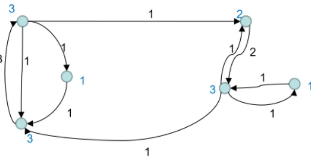
Example 1 (PageRank Graph) Figure 2
shows a graph that is generated from scores {3/13,3/13,3/13,2/13,1/13,1/13}. We omitted the denominators of the scores (of the nodes) and weights (of the edges) in the figure.
Then our divide-and-conquer computation of the backward PageRank by the decompositions=s1⊕s2of node scores is to compute graphsg=g1⊗g2such that
g1 = pr−1 s1
g2 = pr−1 s2
and
pr(g1⊗g2) =s1⊕s2
We divide the backward PageRank computationpr−1fors into computations ofpr−1fors
1ands2(Divide) and obtain
4
Some application may not be interested in the absolute val-ues of scores for individual nodes, so the input can be just a his-togram of scores. This relaxation includes specification of top-k
3
3
1
2
3 1
1
1
1 1
1
3 1
1 1 2
Figure 2: PageRank Graph Example
the entire result (Conquer) by combining the results using ⊗.
4.2
Introduction of virtual nodes
Our graph decomposition is based on the following observa-tions by introducingvirtual nodes. Consider the decomposi-tion of a graphginto two graphsg1andg2by decomposing the set of nodes ofginto two sets. Theng1andg2are created by these nodes, edges that do not cross the boundary of the node sets, and for each subgraph, a virtual node that repre-sents the other subgraph, and edges incoming/outgoing the virtual node that consist of the edges that crosses the bound-ary. Formally, given decomposition of nodesg.V =V1∪V2 for graphgsuch thatprg=s,
g1.V =V1∪ {w1}
g1.E ={(u, v)|(u, v)∈g.E, u∈V1, v∈V1} ∪ {(u, w1)|(u, v)∈g.E, u∈V1, v∈V2} ∪ {(w1, v)|(u, v)∈g.E, u∈V2, v∈V1} andg2given similarly, we have
prg1 =s|V1∪ {w17→sv}
prg2 =s|V2∪ {w27→sv}
wheresv =P(u,v)∈g.E,u∈V1,v∈V2wg(u)
=P(u,v)∈g.E,u∈V2,v∈V1wg(u)
wheredegreeg : g.V → Int def= {v 7→ P(v,u)∈g.E1 | v ∈
g.V}represents the number of outgoing edges for nodev∈
g.V,wg(v) def
=scoreg(v)/degreeg(v)the weight of the node
v for its adjacent nodes and f|S denotes the restriction of
the domain of the function f to the set S. The nodes w1 andw2correspond to the virtual nodes. The (common) score of them is equal to the total flow that is incoming/outgoing from/to one partition to the other. Note that the total score is not equal to 1 anymore for each partition.
This observation implies that the forward computations after decomposition intog1andg2result in the same scores for each subset of the nodes before the decomposition, which enables the divide-and-conquer approach summa-rized as Algorithm 1 by decomposing the nodes into two sets, or equivalently decomposing scores (via split), inde-pendently generate the graphs allocating the score of the vir-tual nodes as the flow of the scores between the sets, and combine the graphs. Indeed, we have, given score partition s=scoreg1⊕scoreg2defined as
scoreg1⊕scoreg2 def
=scoreg1|g1.V1∪scoreg2|g2.V2
with the virtual nodesw1andw2having the common score
sv,
pr((pr−1 s1)⊗(pr−1 s2)) =s
(g1⊗g2).E
def
=
{(u, v)|(u, v)∈g1.E, u6=w1, v6=w1} ∪ {(u, v)|(u, v)∈g2.E, u6=w2, v6=w2} ∪ {(u, vP)|(u, w1)∈g1.E,(w2, v)∈g2.E,
(u′,w1)∈g1.Ewg1(u ′) =wg
2(w2)}
∪ {(u, vP)|(u, w2)∈g2.E,(w1, v)∈g1.E, (u′,w2)∈g2.Ewg2(u
′) =wg 1(w1)}
Note that the flow (score) should be given appropriately for the existence of the PageRank graph. It is also worth not-ing that by recursively decomposnot-ing scores, a partition may include at most two virtual nodes, one of which is already in-troduced during the previous decomposition. Therefore, the virtual nodes are represented as setsVv, and passed topr−1 as an additional argument so that the recursive call can im-pose virtual node conditions to these nodes.
We delegate the base case (PRINV in Algorithm 1) to SMT solvers as described in Section 4.3.
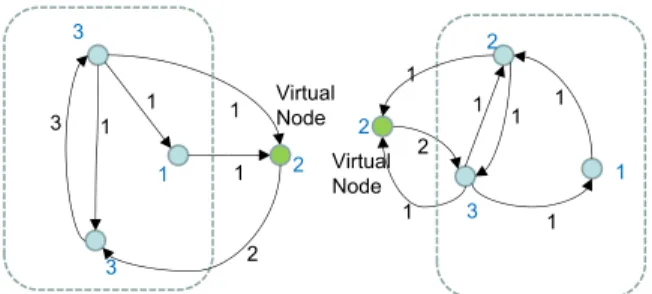
Example 2 (D & C Graph Generation) Figure 3 shows the PageRank graphs g1 and g2 that are generated from scoress1 = {v1 7→ 3/13, v2 7→ 3/13, v3 7→ 1/13, w1 7→ 2/13} and s2 = {v4 7→ 3/13, v5 7→ 2/13, v6 7→ 1/13, w27→2/13}.2/13is chosen as the scoresvof the vir-tual nodesw1andw2. We haves1=prg1ands2 =prg2. Figure 4 shows the graphg1⊗g2.
As a boundary condition around the virtual nodes, the dis-tribution of the weights of the edges incoming to a virtual node, and the distribution of the weights of the edges outgo-ing from the virtual node of the other partition should coin-cide. Alternatively, since there is no restriction in the distri-bution of the incoming edges of a node, if the number of the outgoing edge of a virtual node is only one, then there is no restriction on the incoming edges of the other virtual node. This simplified restriction is applied in the above definition of⊗and used in the constraint to SMT solvers described in Section 4.3.
Example 3 (Boundary Condition) The graphs in Figure 3 satisfies the stronger boundary condition in that the number
Algorithm 1D & C graph generation using virtual nodes
1: procedurepr−1(s, V
v)
2: ⊲generates a graphgs.t.pr g=s
3: ifnondivisibles Vvthen 4: returnPRINV(s, Vv)
5: ⊲generate a graph using SMT solver 6: else
7: ((s1, Vv1),(s2, Vv2))←splits Vv
8: ⊲s.t.s1⊕s2=sfor the virtual nodevv∈Vv 9: g1←pr−1(s1, Vv1)
10: g2←pr−1(s2, Vv2)
3
3 1
2
1 1
1 1 1
1 3 1
1 1
2 2
1 Virtual Node
Virtual Node
2 1
2
3
Figure 3: Divide-and-Conquer Generation of PageRank Graph (flow=2/13)
3
3 1
2
3
1 1
1 1
1
3 1
1 1
1 1
1
Figure 4: Conquer Phase
of outgoing edges in the virtual nodesw1andw2are 1, al-lowing independent generation of PageRank graphs froms1 ands2. Note thats1 ands2should also be in the range of
pr.
4.3
Generation of PageRank graphs in SMT-LIB2
After decomposing input scores to make the number of scores small enough (as determined by the predicate indi-visible in Algorithm 1), we use SMT solvers to generate PageRank graphs (PRINV in Algorithm 1). We show the pseudo-code to represent the input to the solver in Figure 5. The code is similar to that of Figure 1 except that Figure 5 is adapted to the SMT-LIB2 (Barrett, Stump, and Tinelli 2010) standard syntax, introduced the virtual nodes and their boundary conditions (see the comments in the code). The scores of the non-virtual nodes are given by the first set
of assert commands while the scores of virtual nodes are
used by the next set of such commands. The rest of the code fragment, including the boundary conditions are the same for every invocation ofPRINV. The result is extracted as the value assignments of the function edge. Thanks to the standardization by SMT-LIB2, we were able to run the code across multiple platforms including Yices2 (Dutertre 2014), Z3 (De Moura and Bjørner 2008) and CVC4 (Barrett et al. 2011). We use quantifier-free, uninterpreted function with linear integer and real arithmetics (QF UFLIRA) as the con-figuration for the logic and theories.edge v v′
represents the fraction of the score of nodevthat is contributed to nodev′
. Its non-zero value implies the existence of an edge between these nodes. The predicate zeroOrFix represents that the contribution mentioned above is uniform.pagerankCond v represents the PageRank condition for nodevthat ensures
the sum of the contributions from its incoming edges consti-tutes the score ofv, and the sum of the contribution forv’s outgoing edges equals to the score. The predicate weight encodes an existential quantification that ensures uniformity of weights of the edges outgoing from a node. To avoid triv-ial solutions in which every node has only a self-cycle, we add the corresponding condition using function edge. The boundary condition for the virtual nodevvis represented by
rank vv=weightvv, indirectly encodes that the number of outgoing edges is one, so that all the score contributes to the weight.
rank :Node →Real edge :Node×Node →Real weight :Node →Real
assertrank v0=s(v0)
assertrank v1=s(v1) · · ·
assertrank vv1=sv1 (* virtual node *)
assertrank vv2=sv2 · · ·
rank vv1=weightvv1(* boundary condition *)
rank vv2=weightvv2 · · ·
sumInRank :Node →Real sumInRank v=Pv′∈V edgev
′
v edgeOutRange :Node →Bool
edgeOutRange v=Vv′∈V 0≤edge v v
′≤1
sumOutRank :Node →Real sumOutRank v=Pv′∈V edge v v
′
zeroOrFix :Node×Node →Bool
zeroOrFix v n=edge v n= 0∨edge v n=weightv allZeroOrFix Node→Bool
allZeroOrFix v=Vv′∈V zeroOrFix v v
′
pagerankCond :Node→Bool pagerankCond v=
rank v=sumInRank v
∧rank v=sumOutRank v
∧allZeroOrFix v(* uniform weight *) ∧edgeOutRangev(* weight range *) ∧edge v v= 0 (* non-self-cycle *)
assertVv∈V pagerankCondv
Figure 5: SMT Solver inputs
Example 4 shows a generation ofg1in Example 2.
Example 4 (Generation of a Graph in a Partition) V = {0,1,2,3} Vv = {2} s(0) = 3/13, s(1) = 3/13, s(3) = 1/13, s(2) = 2/13 generates edges {(0,1),(0,2),(0,3),(1,0),(2,1),(3,2)}.
Memoization of subgraphs
and reuse the graphs by looking up the graphs needed, by the scaled scores.
Example 5 (Graph Generation by Reusing Memo Entries)
Given scores in Example 1, we can first choose scores *3/13,3/13,2/13+ with flow=1/13, scaling by 13, and reuse the graph at the left bottom of figure 6 for one partition, and graph with scores *3,1,1+ for the other partition, and connect (Figure 7).
2
1 1 1
2 1 1 1 1 1 1 1 2 3 1 1 2 3 1 3 1
2 3 1 1 1 1 2 1 1 1 1 1 1 2 1 2 2 1 2 1 2 1 2 1 1 1 1 1 1 1 2 1 2 2 1 1
2 1 3
1 1 2 2
1 1
1
3
1 1 1
1 1 1 1 (a) (b) (c) (d) (i) (h) (g) (f) (e) (j)
Figure 6: Memo Table for flow=1
{3,3,2} hits in the memo table (flow=1)
2 3
1 1 2 3 1 3 1
{3,1,1} hits
3
1 1 1
1 1 1 1 2 3 1 3 2 3 1 1 3 1 1 1 1 1 1
Connect entries (with no error)
Figure 7: Graph Generation by Reusing Memo Tables
4.4
Discussions
Restrictions on the topology of generated graphs We have introduced a restriction on the boundaries of partitions to enable divide-and-conquer approach, namely, every edge crossing the partitions should be connected to a common node. Natural question here is whether this restriction is re-alistic. We have investigated a real-world graph to see if such partitioning is possible.
Figures 8 and 9 are two different manual partitions of Zachary’s Karate Club (Zachary 1977) that satisfy the re-striction. Though boundary of partitions are not drawn, please consider that nodes placed on the left half of the fig-ure belongs to the left partition and the rest of the nodes be-long to the other partition. By no means these are sufficient to show that the restriction is realistic enough. However, at least we have shown that there exist a graph that can be gen-erated by our D&C approach.
Forward D & C computation by Rescaling scores of sub-graphs As we discussed so far, D & C computation of
Figure 8: Partitioning example (1) of Zachary’s Karate Club (Zachary 1977)
Figure 9: Partitioning example (2) of Zachary’s Karate Club (Zachary 1977)
forward PageRank is generally impossible due to global in-fluence of scores. However, as long as there is a partition that satisfies the boundary constraint, we can independently compute the PageRank of subgraphs including virtual nodes, and then uniformly rescale the scores of each partition so that the score of virtual node coincides and the sum of the ordinary (non-virtual) nodes of both partitions is equal to 1. Suppose the scores of virtual nodes aresv1andsv2for par-tition 1 and 2, respectively, then the scale factorsα1andα2 for each partition are
α1=
sv2
sv2(1−sv1) +sv1(1−sv2)
α2=
sv1
sv1(1−sv2) +sv2(1−sv1)
{1 7→ 1,2 7→ 1}, graph (c) by further superimposing the same graphg, graph (h) by splitting the node with score 2 in graph (b), graph (i) by shifting part of flow (=1) direct-ing to the right to the upper node in graph (h), graph (j) by superimposing graph g to graph (i), graph (b) by sequen-tially connecting graph (a) to itself, and so on. It is our future work to construct memo tables without using SMT solvers efficiently using these basic operations.
5
Graph Generation by Kronecker’s Product
In this section, we show that could reverse iterative queries in a divide-and-conquer manner through finding a matrix satisfying an equation. As we know, many of the iterative computation problems such as PageRank, random walk and graph reachability are formalized as problems for finding an n-dimensional vectorvsatisfyingAv=vfor a givenn×nmatrixAthat is an adjacency matrix of the input graph. Con-trary, in our context where an appropriate input is expected to be generated from an output, we should find a solution that is a matrixAsatisfyingAv = vfor a given vectorv.
Note that the solution is not unique in general and an identity matrix is always a trivial solution. In the PageRank example, the trivial solution corresponds to a graph consisting of only self cycles, which is not desired for our purpose of data gen-eration.
Our goal is to find a nontrivialn×nmatrixAsatisfying Av = v for a givenv. It is so hard in particular whenn,
the number of nodes of the graph, is very large. We give the solution as a Kronecker’s productA=A1⊗ · · · ⊗Akwhere
Ai (i = 1, . . . , k)has almost the same dimension so as to
generate a portable and distributable data.
We design a divide-and-conquer algorithm to find a set of small matrices whose Kronecker’s product is equivalent to a solution Aof Av = v. Suppose that there is a method
for obtainingm-dimensional vectorsv1andv2from a2m
-dimensional vectorvsuch thatv1⊗v2=vholds. We can
find Ai(i = 1,2) satisfying Aivi = vi with a recursive
procedure. ThenA=A1⊗A2is found to satisfyAv=v
since we have
Av= (A1⊗A2)(v1⊗v2) = (A1v1)⊗(A2v2) =v1⊗v2
=v.
We may stop the recursive step at a threshold to switch the other algorithm for finding a small matrix.
The algorithm above cannot be complete to attain our goal, however. The problem is that there may be no vec-tors v1 and v2 such that v = v1 ⊗v2. For example, v = (1 2 2 4)T has a solutionv1 = v2 = (1 2)T, while v= (1 2 3 4)T andv= (1 2 4 2)T have no solution. A
pos-sible approach for evading the problem is to try to minimize kv−v1⊗v2kFwherekxkFdenotes the Frobenius Norm of
a vectorx. In the case ofv= (1 2 3 4)T, we could choose v1 ≈ (0.946 2.138)T andv2 ≈ (1.347 1.911)T to have v1⊗v2≈(1.274 1.808 2.880 4.086)T. Another approach
for the problem is to allow to permutevbefore findingv1
andv2, that is,π(v) = v1⊗v2with a proper permutation
Algorithm 2Kronecker approximation for vectors 1: procedureKRONECKERAPPROX(v)
2: ⊲findsv1andv2s.t.π(v)≈v1⊗v2with someπ 3: v2←a|v|/2-vector whose all values are2/|v| 4: repeat
5: v1←arg minv1kπ(v)−v1⊗v2kF
6: ⊲v2andπfixed
7: v2←arg minv2kπ(v)−v1⊗v2kF
8: ⊲v1andπfixed
9: π←arg minπkπ(v)−v1⊗v2kF
10: ⊲v1andv2fixed
11: until kπ(v)−v1⊗v2kF converges 12: return(v1,v2)
π. In the case ofv= (1 2 4 2)T, one may notice that there
is a solution for its permutation(1 2 2 4)T
. The order can be arbitrary arranged in our purpose when the matrix represents an adjacent matrix
From these observations, we take an approximative ap-proach in which we find vectors v1 andv2 that minimize kπ(v)− v1 ⊗v2kF with varying permutation π.
Algo-rithm 2 shows the procedure which gives a pair of vec-tors v1 and v2 that minimizes kπ(v) −v1 ⊗ v2kF for
a given v varying the permutation π. With π fixed, we
could solve the minimization problem by Singular-Value-Decomposition (SVD) approximation. Let Mv be a
ma-trix such that the vector v is obtained by stacking the
columns ofMv. To minimizekv−v1⊗v2kF for v, an
SVD U1ΣUT
2 of the matrix Mv with diagonal matrix Σ
whose (1,1)-component σ11 is a maximum entry gives a solution (v1,v2) = (σ11u1,u2)whereui is a vector
ob-tained by stacking the columns of Ui (Loan and
Pitsia-nis 1993). The decomposition is known to be achieved by an iterative algorithm of linear procedures (Pitsianis 1997; Johns, Mahadevan, and Wang 2007) as follows:
repeat
v1←arg minv1kv−v1⊗v2kF ⊲v2fixed v2←arg minv2kv−v1⊗v2kF ⊲v1fixed untilkv−v1⊗v2kF converges
Algorithm 2 extends the iterative procedure by varying the permutationπ. To find a better permutation, the same order of the kronecker product of fixed vectors is used.
Using Algorithm 2, it is easy to find a set of matrices de-rive an approximationA ≈A1⊗ · · · ⊗Ak by
divide-and-conquer. Algorithm 3 shows the procedure which derives a matrixAas a Kronecker’s product such thatAv =vfor a
given vectorv.|v|denotes the dimension of the vectorvand
6
Conclusion and future work
This paper reports our work in progress on reversing iter-ative queries for systematic generation of graphs. The key idea is to reduce graph generation as a reverses of a fixed point computation, and to make it scalable through paral-lelization based on the divide-and-conquer approach.
Quite a lot of work is to be done in the future. First, in this paper we consider as an input the complete specification of the problem, like complete list of scores for every nodes in case of PageRank. However some application may require only the stochastic profile of them, like top-kor histogram of scores. We would like to make use of this relaxation to generate graphs more efficiently. Second, the Divide-and-conquer approach may repeatedly produce the same sub-graph at different levels and branches of recursions. We have discussed in Section 4.4 to use memoization to avoid re-computation, but the memo table entries themselves were constructed using SMT solvers. We could instead use com-bination of basic operations to construct these memo tables systematically. Finally, we should seriously implement our new graph generation method and evaluate it with practical graph generations.
References
Aurenhammer, F. 1991. Voronoi diagrams—a survey of a fundamental geometric data structure. ACM Comput. Surv.23(3):345–405.
Barrett, C.; Conway, C. L.; Deters, M.; Hadarean, L.; Jo-vanovi´c, D.; King, T.; Reynolds, A.; and Tinelli, C. 2011. Cvc4. InProceedings of the 23rd International Conference on Computer Aided Verification, CAV’11, 171–177. Berlin, Heidelberg: Springer-Verlag.
Barrett, C.; Stump, A.; and Tinelli, C. 2010. The SMT-LIB Standard: Version 2.0. Technical report, Department of Computer Science, The University of Iowa. Available at
www.SMT-LIB.org.
Binnig, C.; Kossmann, D.; and Lo, E. 2007. Reverse query processing. In Chirkova, R.; Dogac, A.; ¨Ozsu, M. T.; and Sellis, T. K., eds., Proceedings of the 23rd International Conference on Data Engineering, ICDE 2007, The Mar-mara Hotel, Istanbul, Turkey, April 15-20, 2007, 506–515. IEEE.
Algorithm 3Generating a matrixAas a Kronecker’s prod-uct
1: procedureFIXEDPOINTINVERSION(v)
2: ⊲generates a matrixAs.t.Av=v 3: if|v|< σthen
4: GraphGen(s)
5: ⊲call the other algorithm for smaller vectors 6: else
7: (v1,v2)←KRONECKERAPPROX(v)
8: ⊲so thatv1⊗v2≈π(v)with someπ 9: A1←FIXEDPOINTINVERSION(v1)
10: A2←FIXEDPOINTINVERSION(v2) 11: returnA1⊗A2
Capota, M.; Hegeman, T.; Iosup, A.; Prat-P´erez, A.; Erling, O.; and Boncz, P. A. 2015. Graphalytics: A big data bench-mark for graph-processing platforms. In Larriba-Pey, J., and Willke, T. L., eds., Proceedings of the Third Interna-tional Workshop on Graph Data Management Experiences and Systems, GRADES 2015, Melbourne, VIC, Australia, May 31 - June 4, 2015, 7:1–7:6. ACM.
De Moura, L., and Bjørner, N. 2008. Z3: An effi-cient smt solver. In Proceedings of the Theory and Prac-tice of Software, 14th International Conference on Tools and Algorithms for the Construction and Analysis of Sys-tems, TACAS’08/ETAPS’08, 337–340. Berlin, Heidelberg: Springer-Verlag.
Desikan, P. K.; Pathak, N.; Srivastava, J.; and Kumar, V. 2006. Divide and conquer approach for efficient pagerank computation. InProceedings of the 6th International Con-ference on Web Engineering, ICWE ’06, 233–240. New York, NY, USA: ACM.
Dutertre, B. 2014. Yices 2.2. In Biere, A., and Bloem, R., eds.,Computer-Aided Verification (CAV’2014), volume 8559 of Lecture Notes in Computer Science, 737–744. Springer.
He, B.; Yang, M.; Guo, Z.; Chen, R.; Su, B.; Lin, W.; and Zhou, L. 2010. Comet: batched stream processing for data intensive distributed computing. In Proceedings of the 1st ACM Symposium on Cloud Computing, SoCC 2010, Indi-anapolis, Indiana, USA, June 10-11, 2010, 63–74.
Johns, J.; Mahadevan, S.; and Wang, C. 2007. Compact spectral bases for value function approximation using kro-necker factorization. InProceedings of the 22Nd National Conference on Artificial Intelligence - Volume 1, AAAI’07, 559–564. AAAI Press.
Leskovec, J.; Lang, K. J.; Dasgupta, A.; and Mahoney, M. W. 2008. Statistical properties of community structure in large social and information networks. InProceedings of the 17th International Conference on World Wide Web, WWW ’08, 695–704. New York, NY, USA: ACM.
Loan, C. F., and Pitsianis, N. 1993.Linear Algebra for Large Scale and Real-Time Applications. Dordrecht: Springer Netherlands. chapter Approximation with Kronecker Prod-ucts, 293–314.
McCune, R. R.; Weninger, T.; and Madey, G. 2015. Think-ing like a vertex: A survey of vertex-centric frameworks for large-scale distributed graph processing. ACM Comput. Surv.48(2):25:1–25:39.
Nykiel, T.; Potamias, M.; Mishra, C.; Kollios, G.; and Koudas, N. 2010. MRShare: Sharing across multiple queries in mapreduce.PVLDB3(1):494–505.
Onizuka, M.; Kato, H.; Hidaka, S.; Nakano, K.; and Hu, Z. 2013. Optimization for iterative queries on mapreduce.
PVLDB7(4):241–252.
Pitsianis, N. P. 1997. The Kronecker Product in Approx-imation and Fast Transform Generation. Ph.D. Disserta-tion, Cornell University, Ithaca, NY, USA. UMI Order No. GAX97-16143.